How to…
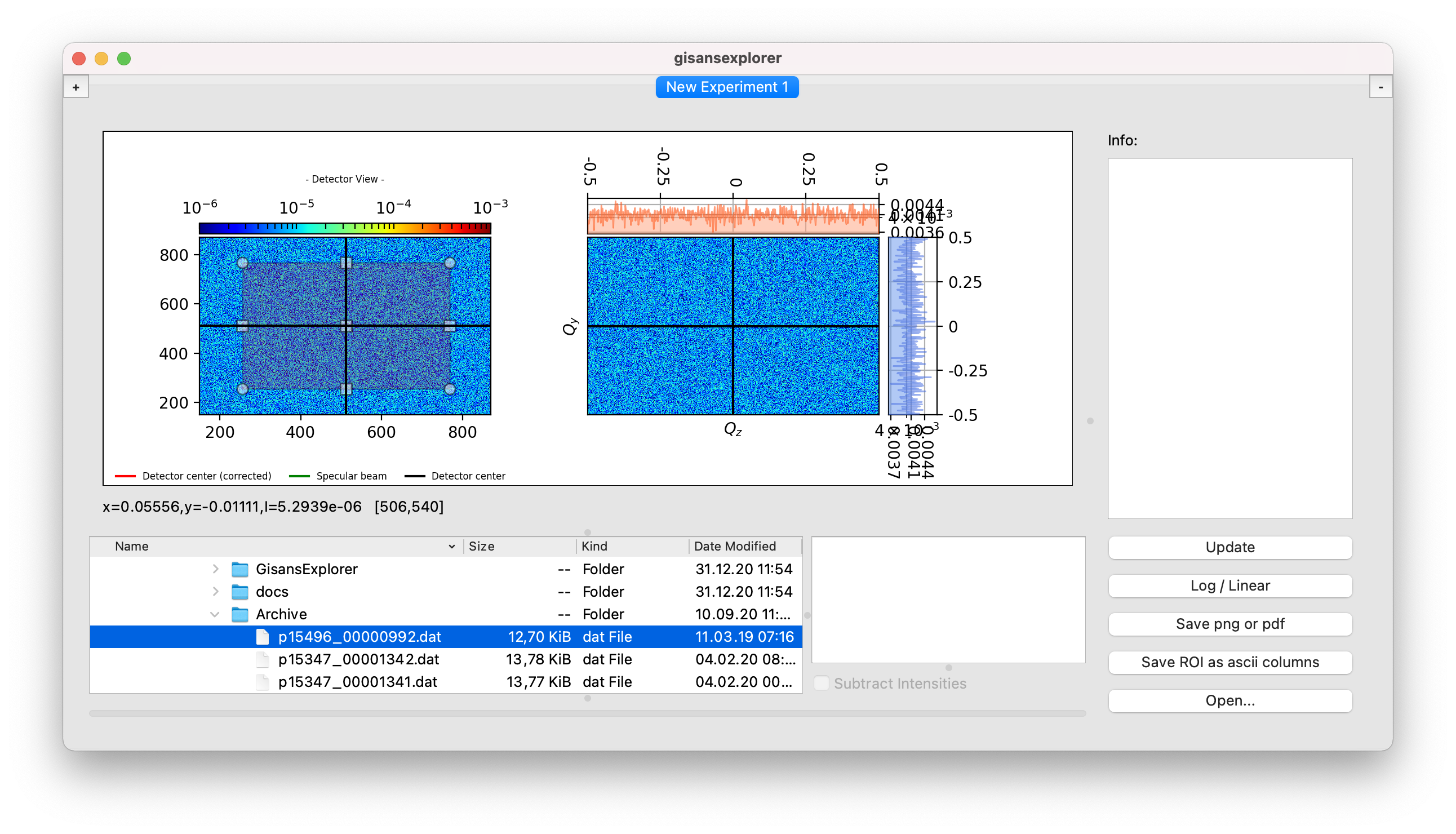
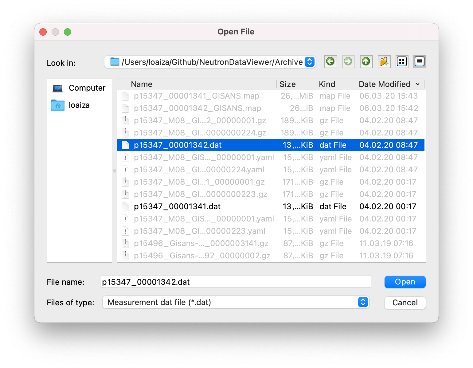
Open a NICOS .dat file
- By navigating to it on the bottom left panel:
- By browsing to it using the open… button on the bottom rigth:
Select the region of interest (ROI)
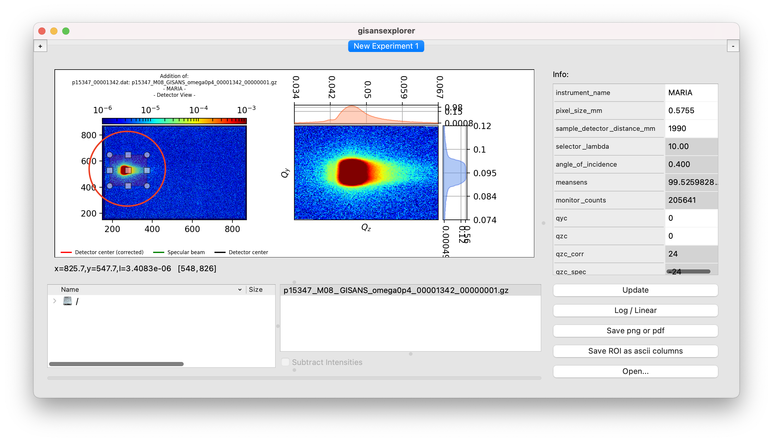
- By using the ROI selector on the left plot:
Click a corner and drag to resize.
Click the center and drag to move.
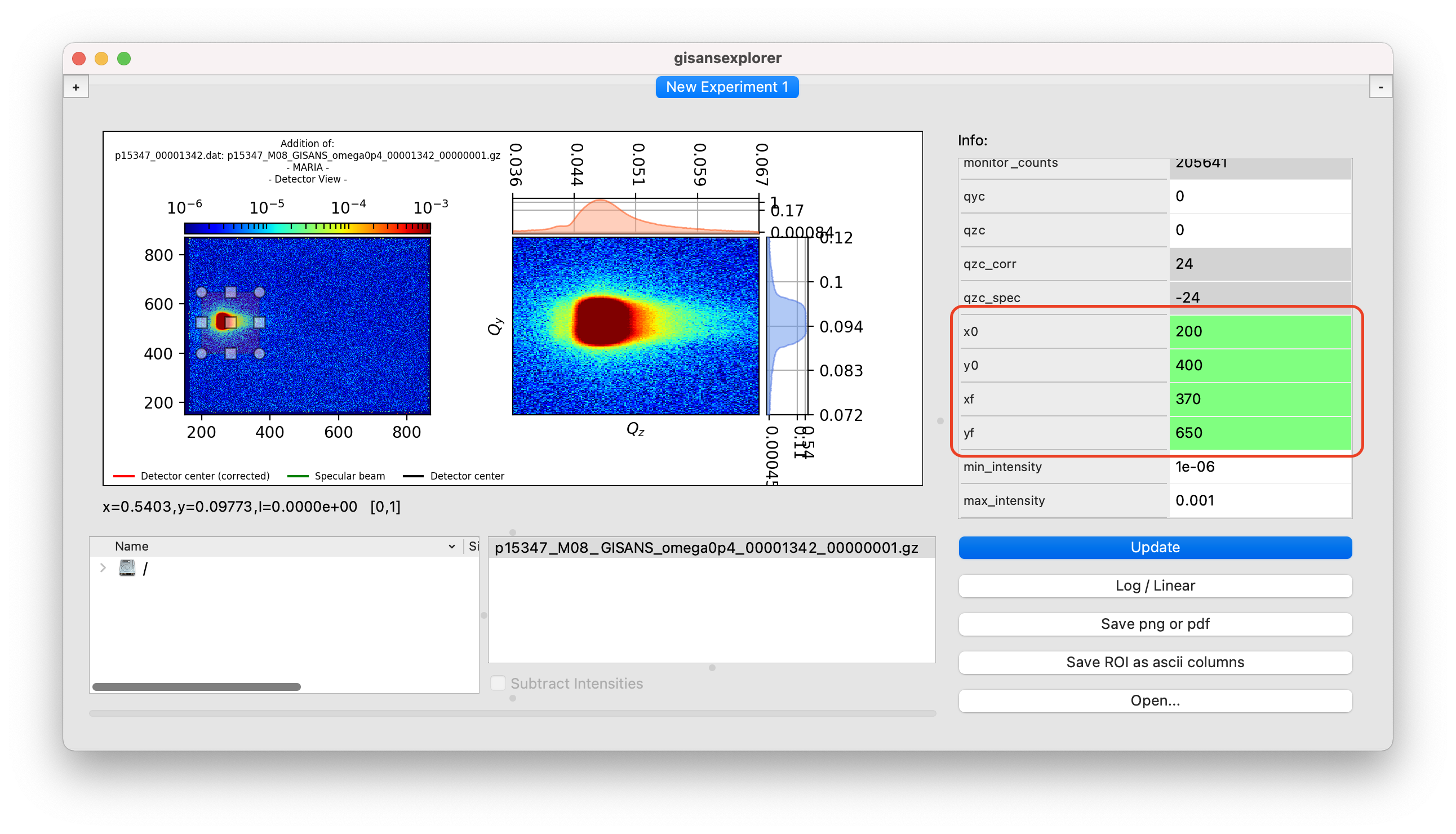
- By setting the limits on the information table on the right:
Set the pixel limit values x0, y0, xf, xf (left, bottom, right, top).
After they turn green –wrong entries will turn red, click Update.
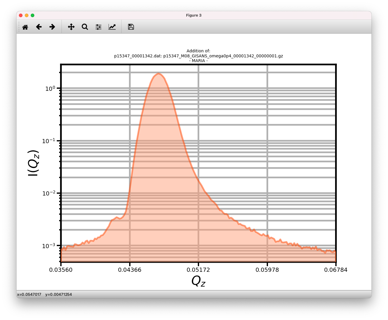
Pop up the ROI plots
By double clicking on any of the ROI plots,
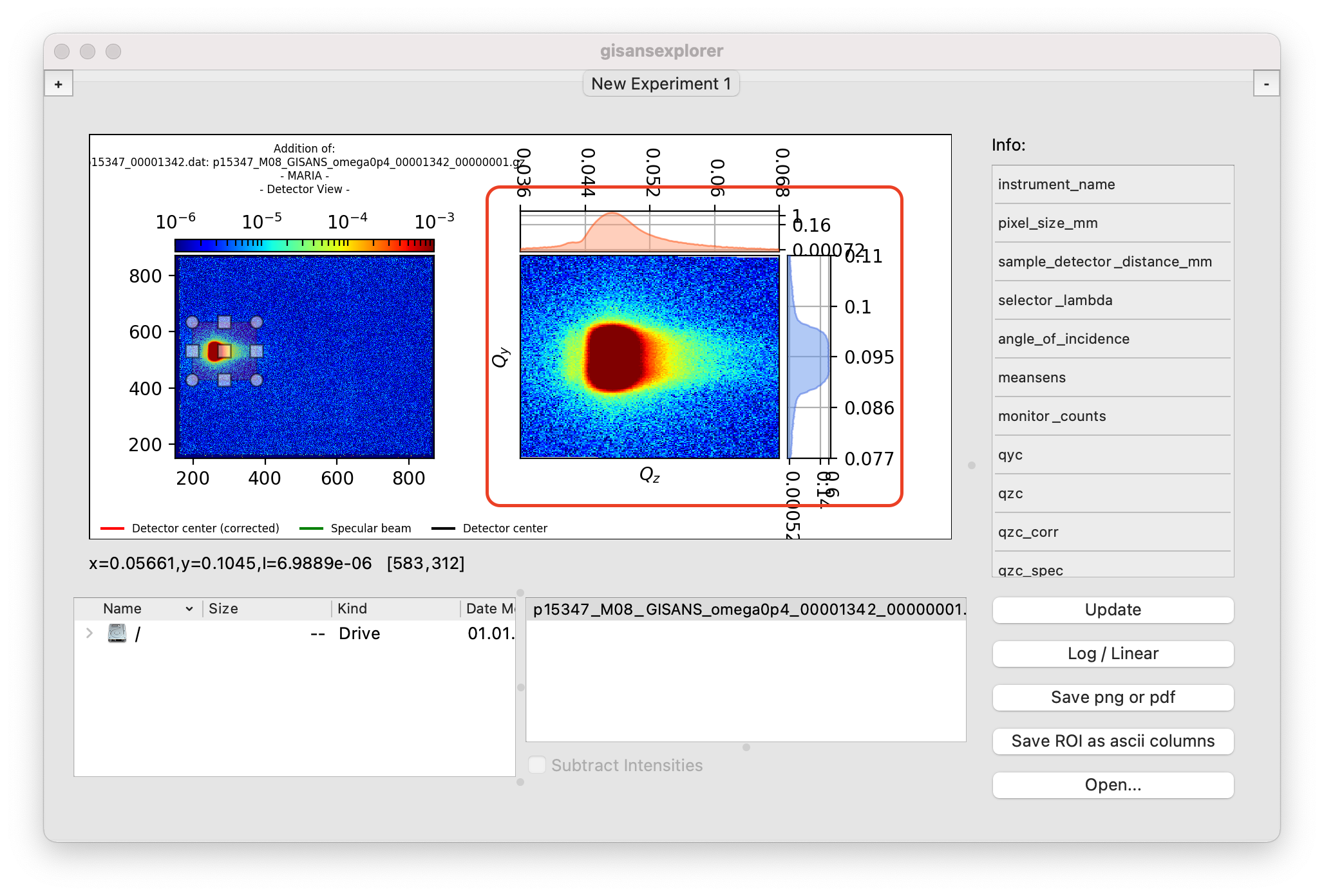 , four pop-up windows will appear:
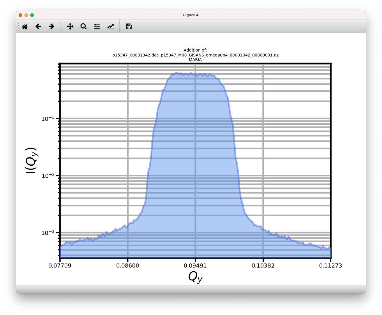
\(Q_z\) vs integration along \(Q_y\)
\(Q_y\) vs integration along \(Q_z\)
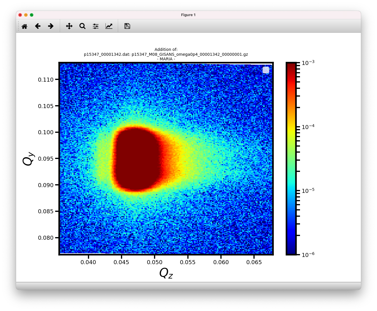
2D Intensity map as function of \(Q_y, Q_z\)
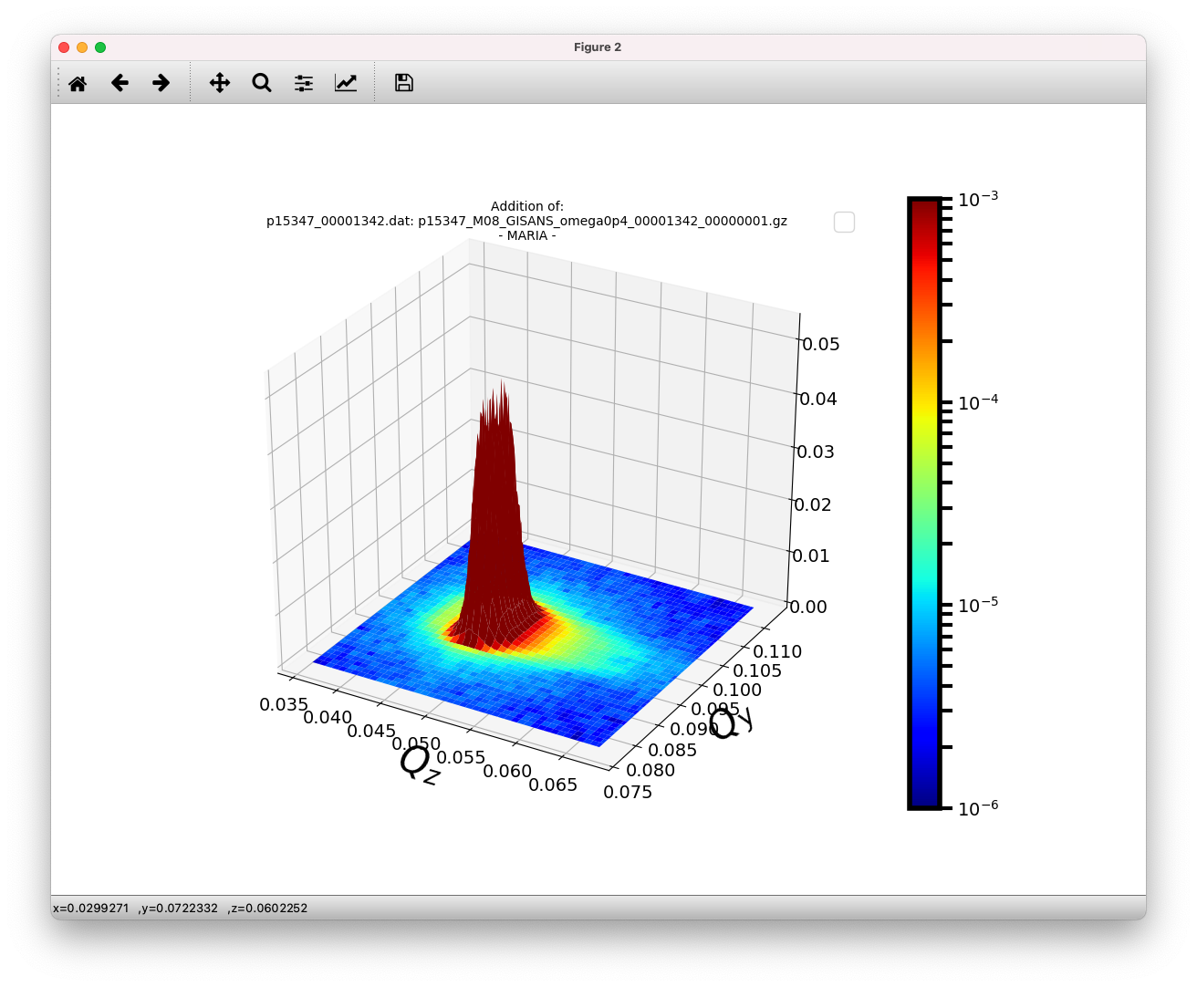
3D Intensity surface as function of \(Q_y, Q_z\)
Clicking the floppy disk icon will save individual figures.
Add or subtract intensities from different Gisans maps
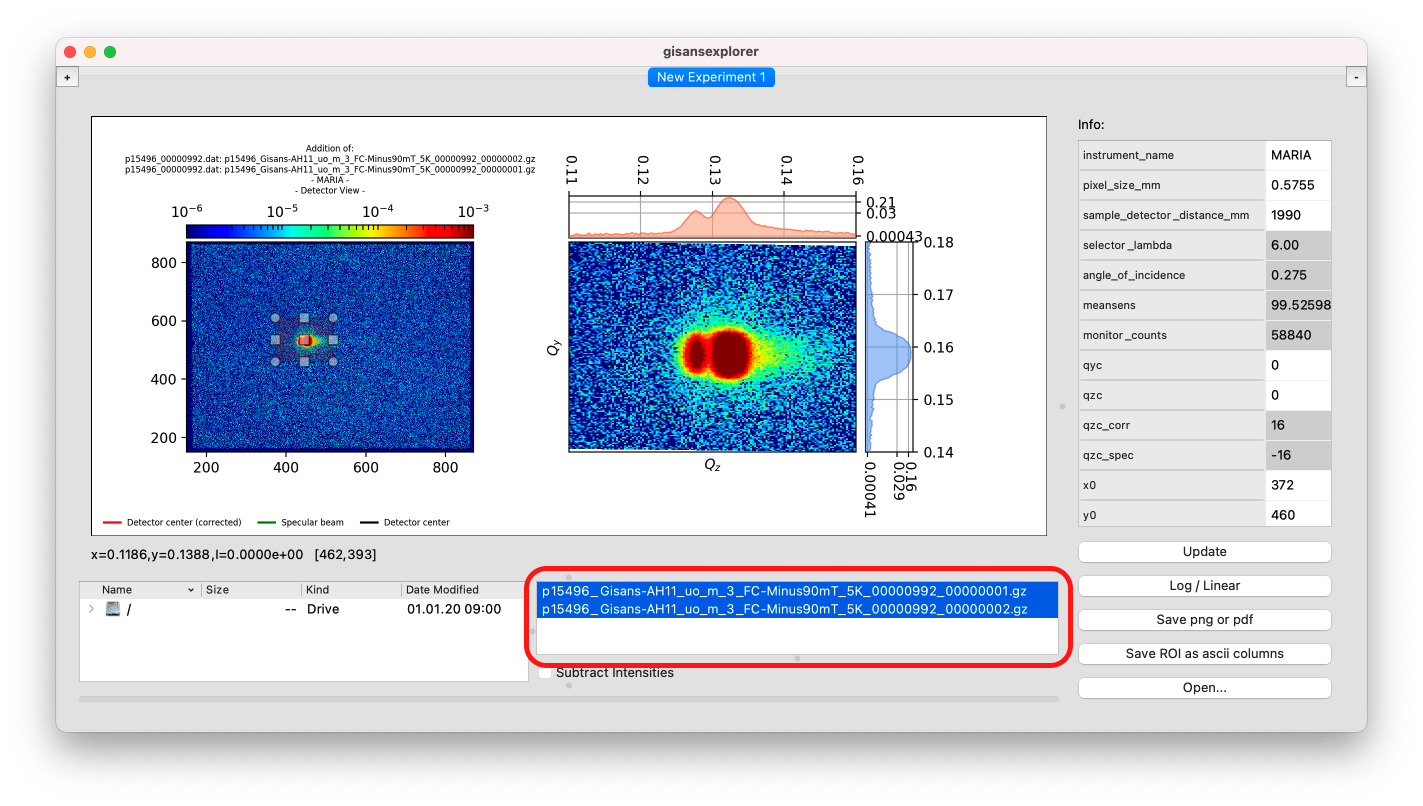
After loading one or more files, click the corresponding maps on the gisans map list. To select several maps, hold the keys
shiftorctrlwhile clicking on each entry. This will automatically show the addition of the intensities of the selected gisans maps. To open several .dat files, repeat the procedure to Open a NICOS .dat file.
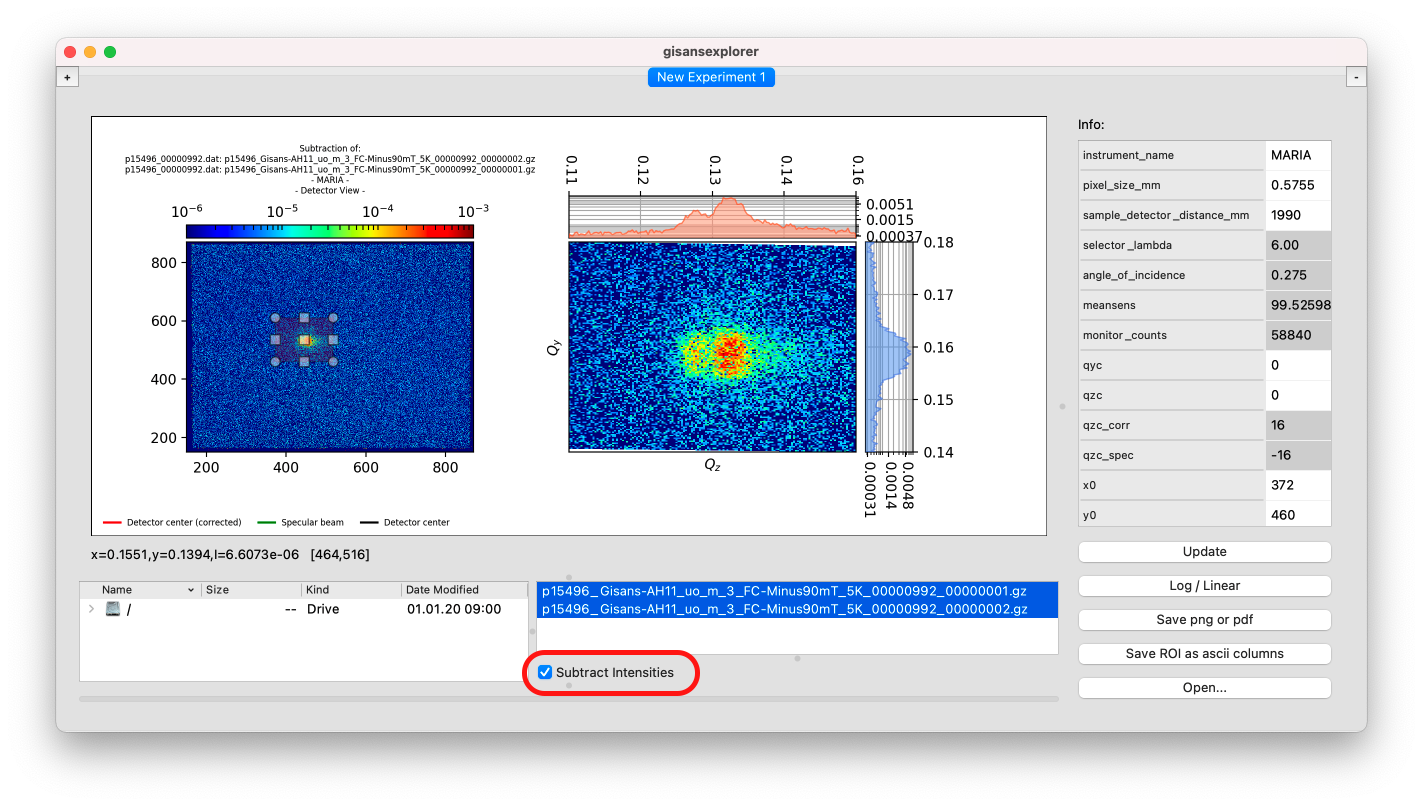
To show the subtraction of the intensities, select any two entries on the list and tick the checkbox Subtract intensities
N.B. While ddition is calculated in the obvious way, \(I = I_A + I_B\), subtraction is calculated as \(I = |I_A - I_B|\).
Save the ROI
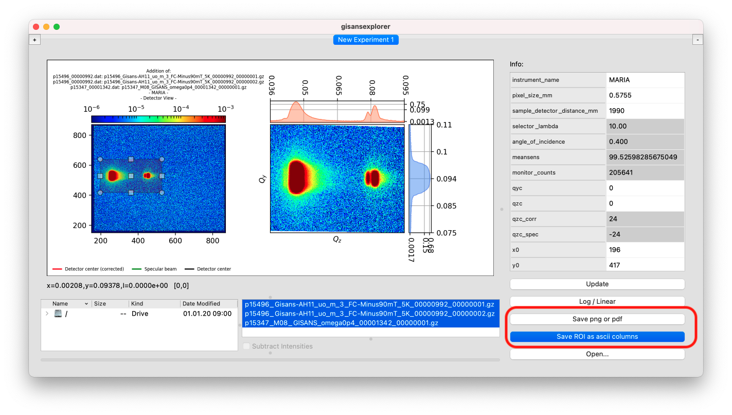
The button Save ROI as ascii columns opens a dialog asking for a location and a filename. After the filename is given (e.g.
MyGivenFilename), three files are saved:MyGivenFilename_xI_.txt- two columns: the first one, the \(x\) coordinate of the detector in \(Q\)-space (i.e. \(Q_z\)); the second one, \(I(Q_z)\), i.e. the intensity integrated along \(Q_y\).MyGivenFilename_yI_.txt- two columns: the first one, the \(y\) coordinate of the detector in \(Q\)-space (i.e. \(Q_y\)); the second one, \(I(Q_y)\), i.e. the intensity integrated along \(Q_z\).MyGivenFilename_xyI_.txt- three columns: analogously to the two previous files, each column represents \(Q_z, Q_y, I(Q_z, Q_y)\).
The button Save png or pdf also opens a dialog asking for a location and a filename. After the filename is given (e.g.
MyGivenFilename), five files are saved:MyGivenFilename.png(or.pdf)MyGivenFilename-integration_qy.png(or.pdf)MyGivenFilename-integration_qz.png(or.pdf)MyGivenFilename-gisans_surface.png(or.pdf)MyGivenFilename-gisans_map.png(or.pdf)
The first file is practically a screenshot of the plotting area,
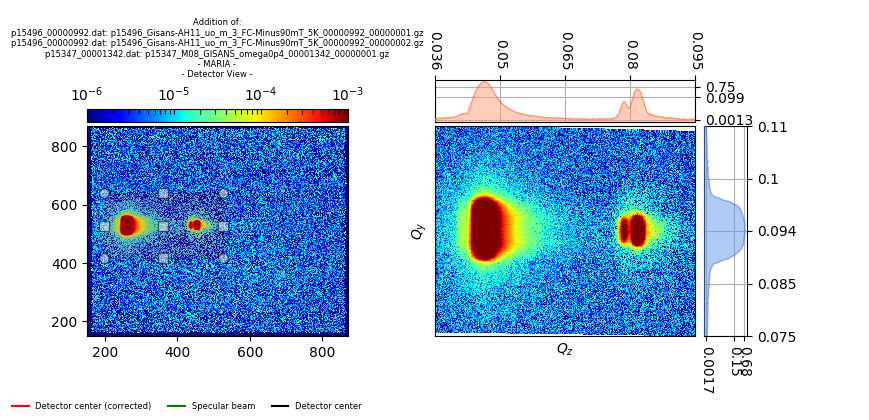
, and the other four files correspond to the figures described in Section Pop up the ROI plots.
Change instrument and detector parameters
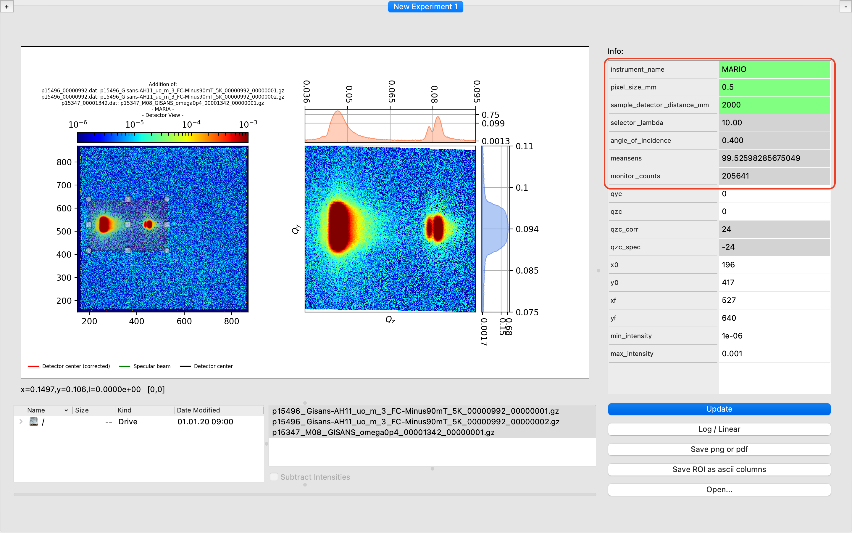
The name of the instrument, the pixel size (in mm) and the sample-detector distance (in mm) can be modified by double-clicking the corresponding entries in the Info table. Once the new entries turn green, the Update button must be clicked for the changes to take effect. the wavelength selector, the angle of incidence, the mean sensitivity, and the monitor counts are read from the NICOS .dat file and thus are not adjustable.
The instrument_name parameter only affects the title of the figures and the header of the ascii file when saving; instead, sample_detector_distance_mm and pixel_size_mm affect also the way in which the \([Q_y, Q_z]\) map is computed for the ROI plot.
Default vaules for the sdd and the pixel size are 1990 and 0.5755 respectively.
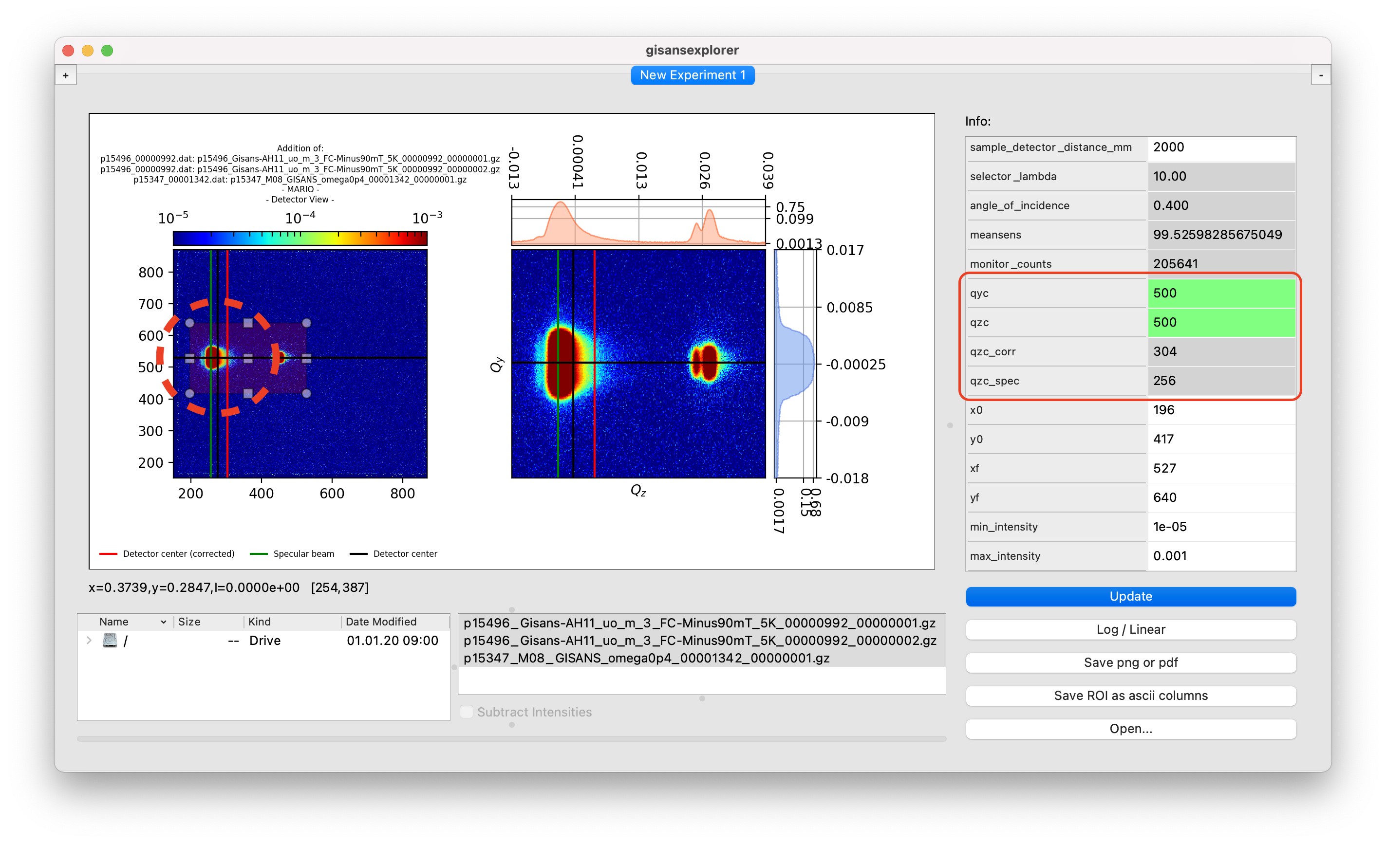
Adjust the beam center position
The detector pixel corresponding to the beam center can be adjusted via the parameters qyc and qzc. By modifying this parameters on the info table, black crosshairs appear on the detector view (left plot) and, if they are inside the ROI, they appear also on the q-space view (right plot). Two additional lines are calculated: a red one, corresponding to the corrected beam center and a green one, corresponding to the specular reflection. For the changes to take effect, the Update button must be clicked after the parameters turn green after being edited.
The location of the green and red lines are properties of the class Experiment and are calculated inside the class MyFrame according to:
experiment.qzc_corr = experiment.qzc + int( ( experiment.sample_detector_distance_mm * np.tan( np.pi * float(experiment.angle_of_incidence) / 180.0) ) / experiment.pixel_size_mm )
experiment.qzc_spec = experiment.qzc - int( ( experiment.sample_detector_distance_mm * np.tan( np.pi * float(experiment.angle_of_incidence) / 180.0) ) / experiment.pixel_size_mm )
Modify the intensity gradient range
The intensity gradient can be shown either in linear scale or in logarithmic scale (default). To switch between these two scales, press the Log/Linear button.
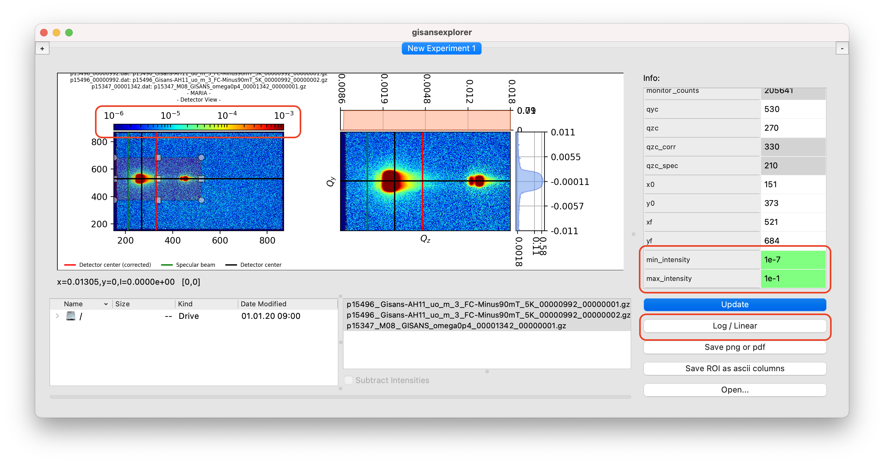
Changing the range of the colormap can be achieved in two ways:
By specifying the minumum and maximum intensity values of the colormap in the Info Table.
By using the mouse wheel while hovering over the detector view (left plot) color bar.
The default min- and max- intensity values are 1e-06 and 1e-03 respectively.
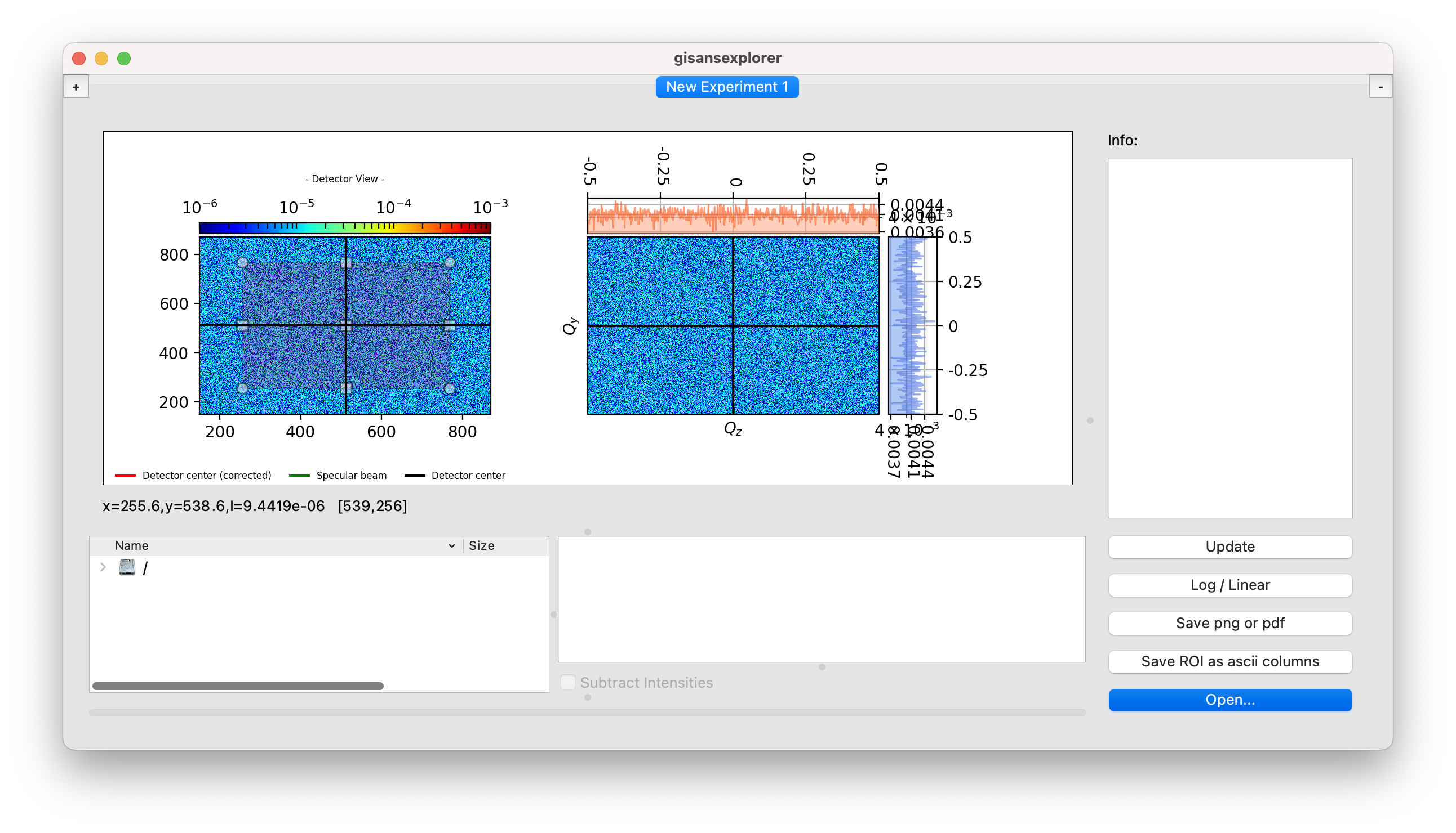
Open and close experiment tabs
Creating new experiments allows to analyse data using different instruments and different sets of parameters in general.
Clicking the left + button will open a new experiment tab.
Clicking the right - button will delete the current experiment tab.
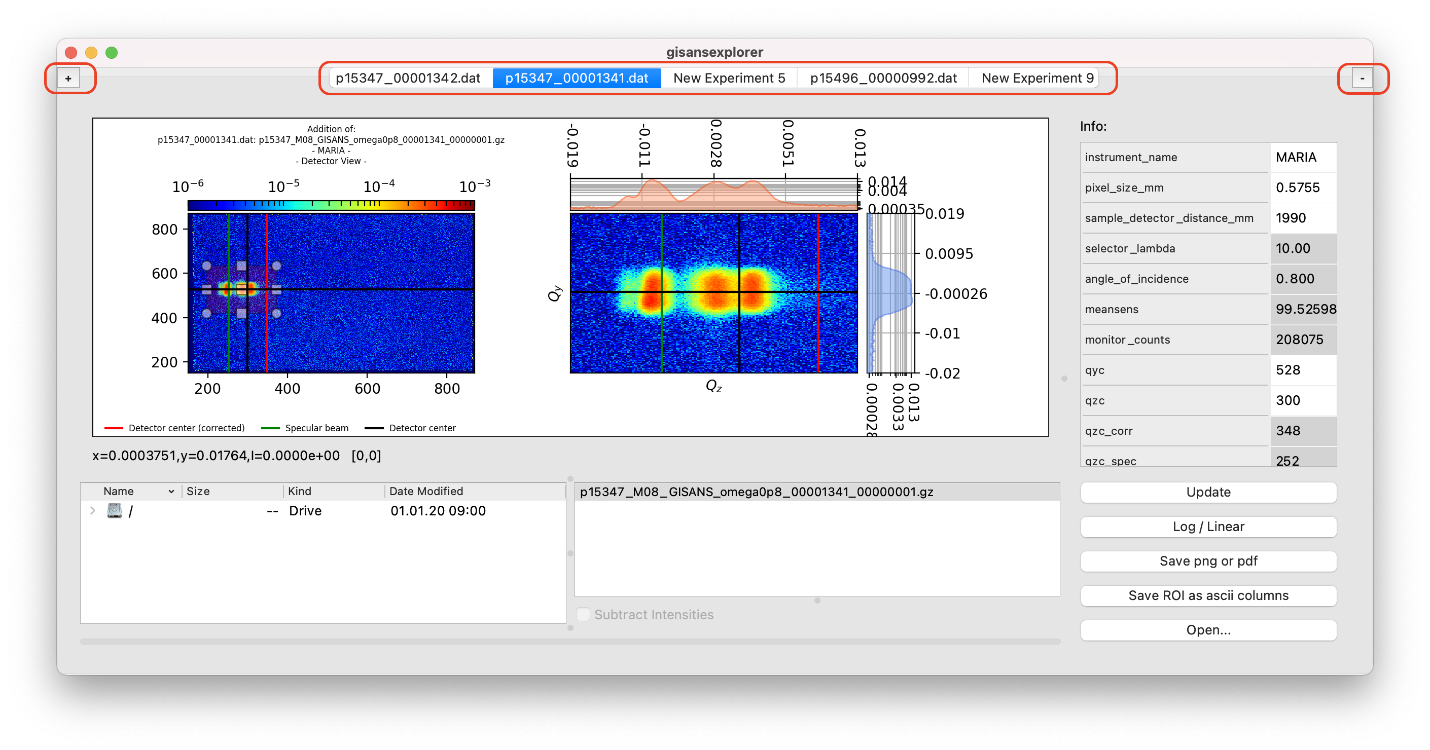
After a new experiment tab is opened, the previous tabs are renamed according to the experimental .dat file opened in them. The new tab will have the default name “New Experiment N”, with N increasing by 1 every time the + button is pressed. The names of experiment tabs are non-editable.
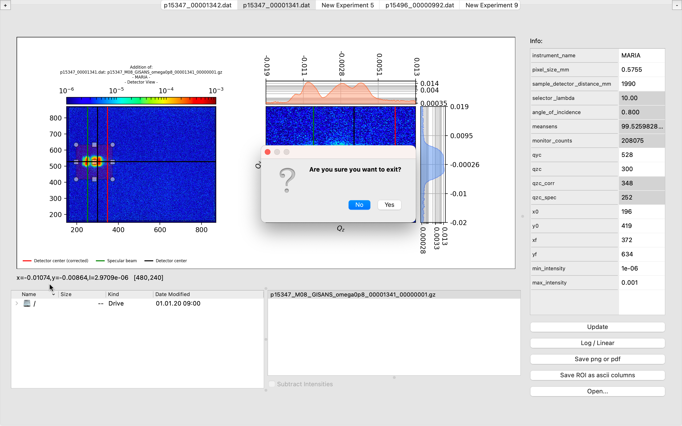
Save progress
Saving the partial progress is not possible. When the close button is pressed (Usually an X in a top corner of the window, depending on the Operating System), a pop-up dialog asks whether to quit the application. After clicking Yes, the application will close and all progress will be lost. Make sure that all the reduced ascii data and the figures required are correctly saved before closing the application –refer to sections Pop up the ROI plots and Save the ROI.